Introducing Connector Private Networking: Join The Upcoming Webinar!
Crossing the Streams – Joins in Apache Kafka
Get started with Confluent, for free
Watch demo: Kafka streaming in 10 minutes
This post was originally published at the Codecentric blog with a focus on “old” join semantics in Apache Kafka versions 0.10.0 and 0.10.1.
Version 0.10.0 of the popular distributed streaming platform Apache KafkaTM saw the introduction of Kafka’s Streams API. In its initial release, the Streams API enabled stateful and stateless Kafka-to-Kafka message processing using concepts such as map, flatMap, filter, or groupBy that many developers are familiar with these days. In Kafka 0.10.1, Kafka Streams started to support “Interactive Queries”, an API that allows querying stateful stream transformations without going through another Kafka topic.
In this article, we will talk about a specific kind of streaming operation – the joining of streams. Kafka Streams improved its join capabilities in Kafka 0.10.2+ with better join semantics and by adding GlobalKTables, and thus we focus on the latest and greatest joins available. We will begin with a brief walkthrough of some core concepts. Then we will take a look at the kinds of joins that the Streams API permits. Following that, we’ll walk through each possible join by looking at the output of an established example. At the end, you should be aware of what kinds of joins are possible in Kafka Streams, including their detailed semantics. This will enable you to leverage the right join in your Kafka Streams application.
A brief introduction to some core concepts
The central component of Kafka is a distributed message broker where producers send messages—key-value pairs—to topics which in turn are polled and read by consumers. Each topic is partitioned, and the partitions are distributed among brokers. The excellent Kafka documentation explains it best.
There are two main abstractions in the Streams API: A KStream is a stream of key-value pairs—a similar model as used for a Kafka topic. The records in a KStream either come directly from a topic or have gone through some kind of transformation—for example there is a filter method that takes a predicate and returns another KStream that only contains those elements that satisfy the predicate. KStreams are stateless, but they allow for aggregation by turning them into the other core abstraction: a KTable, which is often described as a “changelog stream.” A KTable holds the latest value for a given message key and reacts automatically to newly incoming messages.
A nice example that juxtaposes KStream and KTable is counting visits to a website by unique IP addresses. Let’s assume we have a Kafka topic containing messages of the following type: (key=IP, value=timestamp). A KStream contains all visits by all IPs, even if the IP is recurring. A count on such a KStream sums up all visits to a site including multiple visits from the same IP. A KTable, on the other hand, only contains the latest message and a count on the KTable represents the number of distinct IP addresses that visited the site.
KTables and KStreams can also be windowed for aggregations and joins, respectively (i.e., a windowed aggregation produces a windowed KTable as a result while two KStreams can be joined based on a time window; however, KTables joins are none-window-joins). Regarding the example, this means we could add a time dimension to our stateful operations (either an aggregation or a join). To enable windowing, Kafka 0.10 changed the Kafka message format to include a timestamp. This timestamp can either be CreateTime or AppendTime. CreateTime is set by the producer and can be set manually or automatically. AppendTime is the time a message is appended to the log by the broker. The applied time semantic is a broker side topic-level configuration and if AppendTime is set the broker will overwrite the timestamp that is provided by the producer. Next up: joins.
Joins
Taking a leaf out of SQLs book, Kafka Streams supports three kinds of joins:
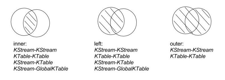
Inner Joins: Emits an output when both input sources have records with the same key.
Left Joins: Emits an output for each record in the left or primary input source. If the other source does not have a value for a given key, it is set to null.
Outer Joins: Emits an output for each record in either input source. If only one source contains a key, the other is null.
Another important aspect to consider are the input types. The following table shows which operations are permitted between KStreams and KTables:
| Primary Type | Secondary Type | Inner Join | Left Join | Outer Join |
| KStream | KStream | Supported | Supported | Supported |
| KTable | KTable | Supported | Supported | Supported |
| KStream | KTable | Supported | Supported | N/A |
| KStream | Global KTable | Supported | Supported | N/A |
As the table shows, all joins are permitted between equal types. An outer join between a KStream and either a KTable or GlobalKTable are the only inter-type joins that are not supported. For more details about global KTables we refer to the documentation and the corresponding KIP-99. A quick explanation is that a global KTable is replicated, in contrast to a “regular” KTable that is sharded. Hence, a global KTable has a full copy of the data and thus allows for non-key joins and avoids data repartitioning for multiple consecutive joins; it’s very well suited for “star joins” with a fact-stream and multiple dimension KTables, similar to star joins in a data warehouse. Another important difference between a KTable and a GlobalKTable is time synchronization: while processing KTable records is time synchronized based on record timestamps to all other streams, a GlobalKTable is not time synchronized. We refer to sections “KStream-KTable Join” and “KStream-GlobalKTable Joins” for details.
From the table above, there are ten possible join types in total. Let’s look at them in detail.
Example
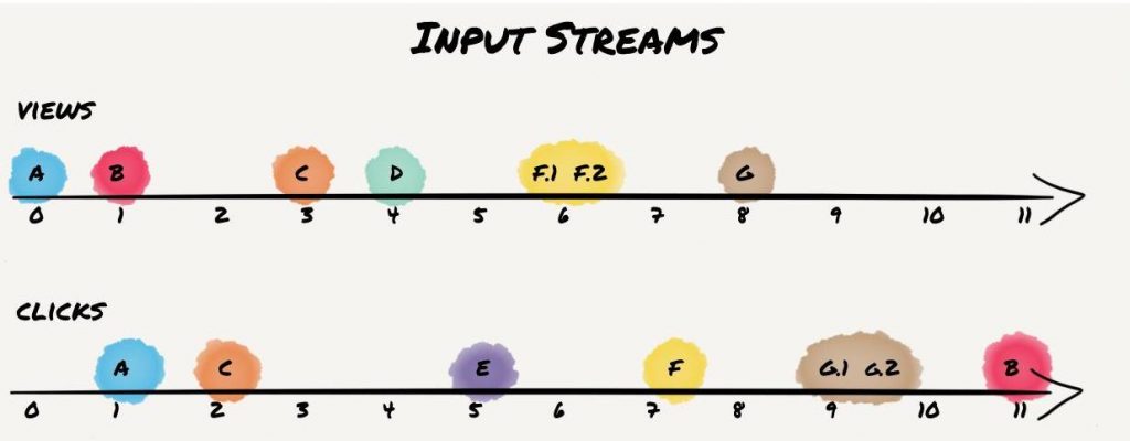
We are going to use an example to demonstrate the differences in the joins. It is based on the online advertising domain. There is a Kafka topic that contains view events of particular ads and another one that contains click events based on those ads. Views and clicks share an ID that serves as the key in both topics.
In the examples, custom set event times provide a convenient way to simulate the timing within the streams. We will look at the following 7 scenarios:
- a click event arrives 1 sec after the view
- a click event arrives 11 sec after the view*
- a view Event arrives 1 sec after the click
- there is a view event but no click
- there is a click event but no view
- there are two consecutive view events and one click event 1 sec after the first view
- there is a view event followed by two click events shortly after each other
*Note that the figures below depicting the B click record at 11 seconds are incorrect and should be at 12 seconds.
This visualization shows these streams: we have two timelines, one for each input stream. We only show the key for each record indicated by a letter. If the same key appears multiple times we extend it with a number suffix (e.g., “F.1”). We also color-coded the records according to the scenarios described above. The time is annotated in seconds.
Inner KStream-KStream Join
All KStream-KStream joins are windowed, so the developer has to specify how long that window should be and if the relative order of the elements of both streams matters (i.e., happens before/after semantics). The rationale behind that forced windowing is twofold: First, a KStream is stateless. To execute a join with acceptable performance, some internal state needs to be kept—otherwise both streams would need to be scanned each time a new element arrives. That state contains all elements of the stream within the time window. Second, semantically speaking, joining two streams yields “interesting” results if both records in each stream are timed close to each other (i.e., both events happened within a certain time frame). For example, an ad was displayed on a web page and a user clicks on it within 10 seconds. Note that the join window is based on event time.
We will use a window of 10 seconds in the following examples.
An inner join on two streams yields a result if a key appears in both streams within the window. Applied to the example, this produces the following results:
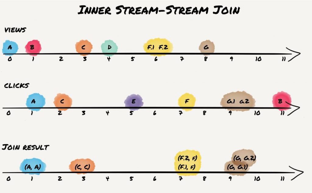
Records A and C appear as expected as the key appears in both streams within 10 seconds, even though they come in different order. Records B produce no result: even though both records have matching keys, they do not appear within the time window. Records D and E don’t join because neither has a matching key contained in both streams. Records F and G appear two times as the keys appear twice in the view stream for F and in the clickstream for scenario G.
In general, join windows for stream-stream joins are symmetric, i.e., allow the record of the other stream to be in the past or in the future (cf. A vs. C with flipped arrival order). Two variations of this are the enforcement of ordering. The developer can specify that a click event can only be joined if it occurs after (or before) a view event. The “after” setting would lead to the elimination of (C,C) result record in our example.
Note that the shown results assume that all records are processed in timestamp order. This might not hold in practice as time synchronization between different streams follows a best-effort approach (though time synchronization was improved in the 2.1.0 release; confer the section about stream-table joins below for more details). However, for inner KStream-KStream joins, this runtime dependency has no impact on the result, which will always be the same. It might have an impact on the order of output records, but nothing more.
Left KStream-KStream Join
While all joins in Kafka are based on event time, left joins have an additional runtime dependency on processing order that yield results that do differ from SQL semantics. One important takeaway is: stream join semantics are not the same as SQL (i.e., batch) semantics.
The left join starts a computation each time an event arrives for either the left or right input stream. However, processing for both is slightly different. For input records of the left stream, an output event is generated every time an event arrives. If an event with the same key has previously arrived in the right stream, it is joined with the one in the primary stream. Otherwise it is set to null. On the other hand, each time an event arrives in the right stream, it is only joined if an event with the same key arrived in the primary stream previously. With our examples, this is going to result in four result records one might not expect if not familiar with the provided semantics. It leads to the following result:
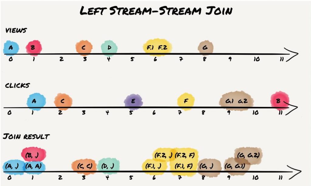
As expected, the result contains all records from the inner join. Additionally, it contains a result record for B and D and thus contains all records from the primary (left) “view” stream. Also note the results for “view” records A, F.1/F.2, and G with null (indicated as “dot”) on the right-hand side. Those records would not be included in a SQL join. As Kafka provides stream join semantics and processes each record when it arrives, the right-hand window does not contain a corresponding keys for primary “view” input events A, F1./F.2, and G in the secondary “click” input stream in our example and thus correctly includes those events in the result.
Similar to inner KStream-KStream join, the shown result matches the shown processing order that aligns with the event time of the events. However, Streams cannot guarantee to process all events according to event time and thus, the result might be slightly different for multiple runs. Nevertheless, this only affects the output records that are different from SQL semantics. It is guaranteed that the result contains all result records from the inner join, as well as all records from the primary stream. To be more precise, due to the described runtime/processing dependency, for each result record that is also an inner join result, there might be one or multiple left join results with null at the right-hand side.
Outer KStream-KStream Join
An outer join will emit an output each time an event is processed in either stream. If the window state already contains an element with the same key in the other stream, it will apply the join method to both elements. If not, it will only apply the incoming element.
It leads to the following result:
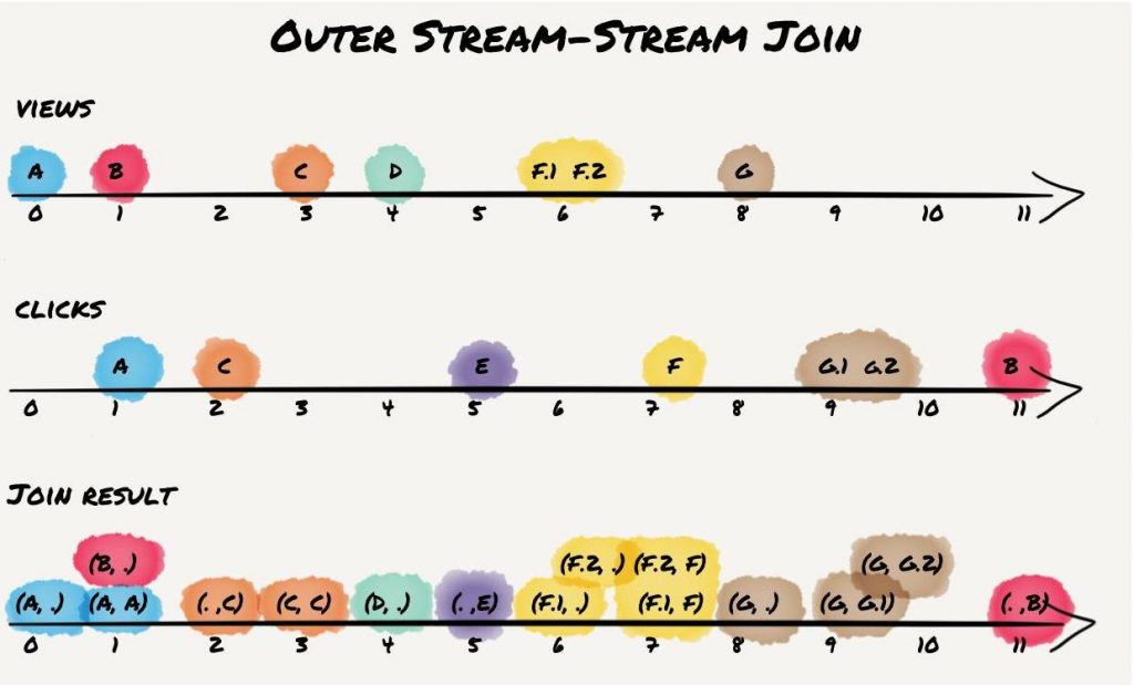
For record A, an event is emitted once the view is processed. There is no click yet. When the click arrives, the joined event on view and click is emitted. For records B, we also get two output events. However, since the events do not occur within the window, neither of these events contains both view and click (i.e., both are independent outer-join results). “View” record D appears in the output without a click, and the equivalent (but “reverse”) output is emitted for “click” record E. Records F produce 4 output events as there are two views that are emitted immediately and once again when they are joined against a click. In contrast, records G produce only 3 events as both clicks can be immediately joined against a view that arrived earlier.
Thus, outer join semantics are similar to left join semantics; however, it’s a symmetric join, and it preserves records from both input streams. Similar to the left join, there is a runtime dependency with regard to the join result with no matching event in the other stream.
Inner KTable-KTable Join
Now we’re switching from KStreams to KTables. A KTable is a changelog stream of updates—thus, a “plain” KTable is a stateless stream with different semantics than a KStream. However, often KTables are also materialized into a local state store, building a table that always contains the latest value for a key. If two KTables are joined they are always materialized. This allows to lookup matching join records. Joins on KTables are not windowed and their result is an ever-updating view of the join result of both input tables. If one input table is updated, the resulting KTable is also updated accordingly; note that this update to the result table is a new output record only, because the resulting KTable is not materialized by default.
The following chart shows results if we interpret both streams as changelogs. It also shows the current materialized table after each update for each input stream:
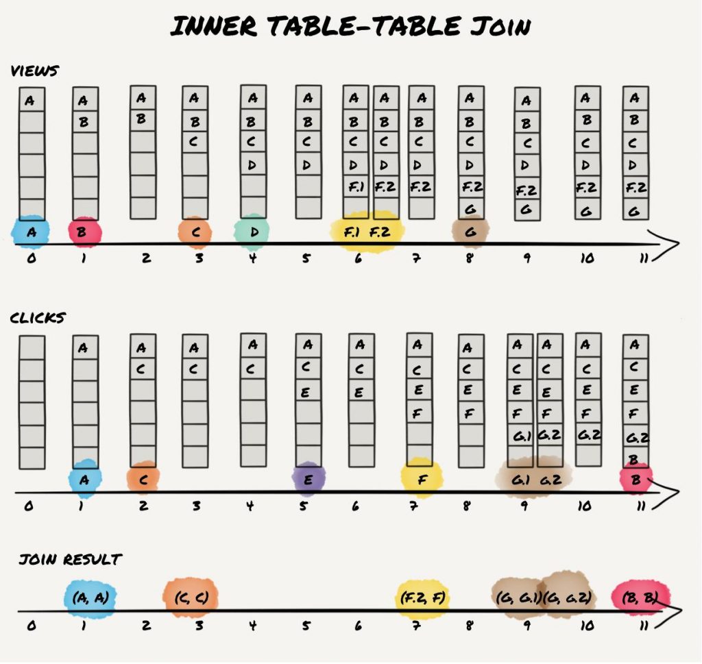
All the inner join pairs are emitted as expected. Since we’re no longer windowed, even record B/B is in the result. Note, that the result contains only one result for F but two for G. Because click F appears after views F.1 and F.2, F.2 did replace F.1 before F triggers the join computation. For G, the view arrives before both clicks and thus, G.1 and G.2 join with G. This scenario demonstrates the update behavior of table-table join. After G.1 arrived, the join result is G.1/G. Then the click event G.2 updates the click table and triggers a recomputation of the join result to G.2/G.1
We want to point out that this update behavior also applies to deletions. If, for example, one input KTable is directly consumed from a compacted changelog topic and a tombstone record is consumed (a tombstone is a message with format <key:null> and has delete semantics), a result might be removed from the resulting KTable. This is indicated by appending a tombstone record to the resulting KTable.2
Last but not least, similar to our KStream-KStream examples, we assume that records are processed in timestamp order. In practice, this might not hold as time synchronization between streams or tables is based on a best-effort principle. Thus, the intermediate result might differ slightly. For example, click F might get processed before views F.1 and F.2 even if click F has a larger timestamp. If this happens, we would get an additional intermediate result F.1/F before we get final result F.2/F. We want to point out that this runtime dependency does only apply to intermediate but not to the “final” result that is always the same.
Left KTable-KTable Join
Left joins also work the way you’d expect by now:
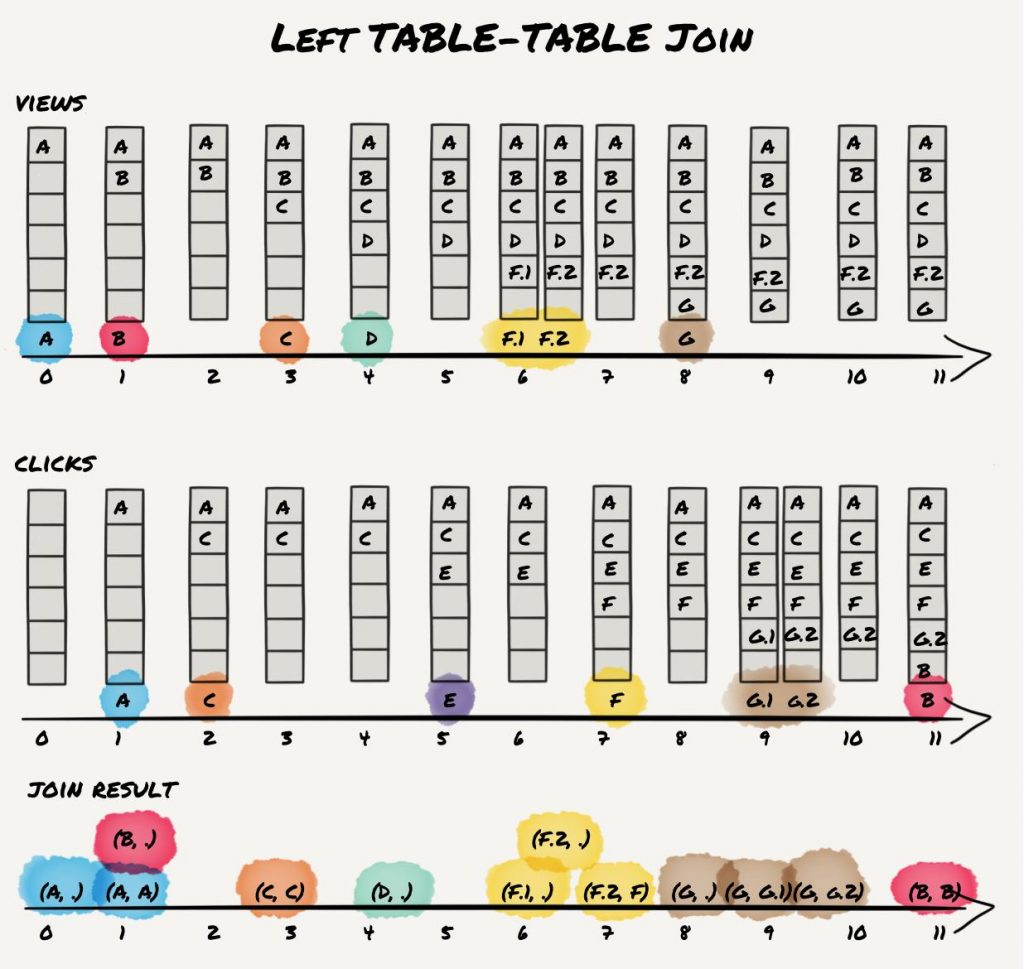
The result is the same as with the inner join with the addition of proper data for (left) view events A, B, D, F.1, F.1, and G that do a left join with empty right-hand side when they are processed first. Thus, view D is preserved and only click E is not contained as there is no corresponding view.
Outer KTable-KTable Join
Outer joins don’t yield any different behavior. It’s an left- and right-outer join at once:
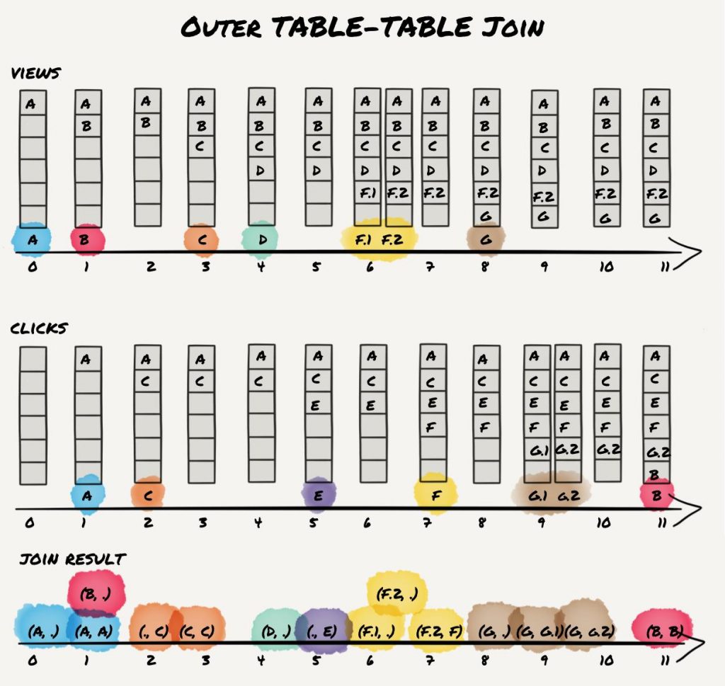
The result is the same as with the left join plus the “right join” result records for clicks C and D with an empty left-hand side.
This concludes the KTable-KTable section. We can observe that KTable-KTable join is pretty close to SQL semantics and thus easy to understand. The difference to plain SQL is that the resulting KTable gets updated automatically if an input KTable is updated. Thus, the resulting KTable can be described as an ever-updating view of the table join. The important aspect here is that the settings for caching play a role in the emission of events from a joined KTable. Yet the end result is the same: each joined KTable has the same content after completely processing the sample data, cached or non-cached.
Inner KStream-KTable Join
Using a stream-table join, incoming events in a stream can be joined against a table. Similar to a table-table join, this join is not windowed; however, the output of this operation is another stream, and not a table. In contrast to stream-stream and table-table join which are both symmetric, a stream-table join is asymmetric. By “symmetric” we mean that the arrival of each input (i.e., left or right) triggers a join computation and thus can result in a result record. However, for stream-table joins, only the (left) stream input triggers a join computation while (right) table input records only update the materialized table. Because the join is not-windowed, the (left) input stream is stateless and thus, join lookups from table record to stream records are not possible. The concept behind this semantics is the idea to enrich a data stream with auxiliary information. For example the stream could contain a user ID and the table has the user ID as key and user information as value. Thus, the stream can be enriched with the full user profile by doing a table lookup on the user ID. Our previous example with the views and clicks does not really work well as you’d probably not use a stream-table join for this. However, to avoid introducing a new example, we’ll just reuse the same data with the view as the left stream input and clicks as the right table input:
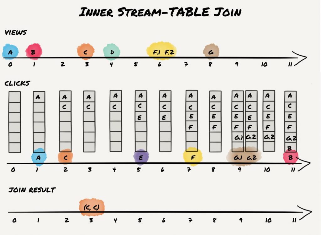
In 2.0.x and older releases, the result is just a single record as click C is the only click that arrives before the corresponding view event. As for KStream-KStream and KTable-KTable joins, there is a runtime dependency on actual processing order. While for KStream-KStream and KTable-KTable joins, this runtime dependency has no big impact on the result, for KStream-KTable joins, it can be notable. The reason is that a KStream-KTable join is asymmetric, as mentioned in the beginning of this section. Thus, if a KStream record is accidently processed before a KTable record that actually does have a smaller timestamp than the KStream record, the join result gets lost. For symmetric joins this cannot happen, as both sides trigger a join computation.
Since the 2.1.0 release, timestamp synchronization has improved and Kafka Streams provides stricter guarantees with regard to processing records based on their timestamps: overall, pick the “partition head” record with the smallest timestamp for processing (see KIP-353). This timestamp comparison can only be done if data is available for all input partitions. To avoid infinite blocking if one input is empty, Kafka Streams now waits until the configured wait time of `max.task.idle.ms` has passed (default is zero, i.e,. don’t block at all what is similar behavior as in older releases) to see if new data may arrive. If no new data arrives within this timeout, processing will just continue based on the available input data. Thus, the result from our example may actually be different depending on which version you are using and what your configuration is. With corresponding temporary blocking, records A, F, and G (and maybe even B) might also produce a join result depending on their event timestamp. If we assume that the arrival/processing timestamp is the same as the event timestamps as shown in our example, the same result as depicted would be computed over all releases.
Left KStream-KTable Join
A left KStream-KTable join behaves straightforwardly with regard to the join semantics we discussed so far. It’s the same as an inner KStream-KTable join but preserves all (left) stream input records in case there is no matching join record in the (right) KTable input:
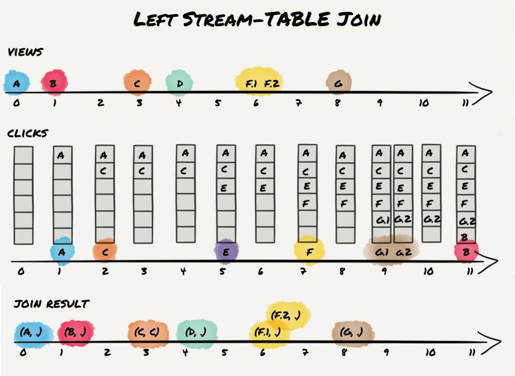
As expected, we get the inner C/C join result as well as one join result for each (left) stream record.
Inner KStream-GlobalKTable Join
The last join we want to cover is KStream-GlobalKTable join. It is basically the same join as a KStream-KTable join. However, it yields different results because a GlobalKTable has different runtime behavior from a KTable.3 First, a GlobalKTable is completely populated before any processing is done. At startup, the GlobalKTables input topic’s end offsets are read and the topic is read up to this point populating the GlobalKTable before any processing starts. Second, if new updates are written to the GlobalKTables input topic, those updates are applied directly to the materialized table. With regard to our example and an inner KStream-GlobalKTable join we get the following result:
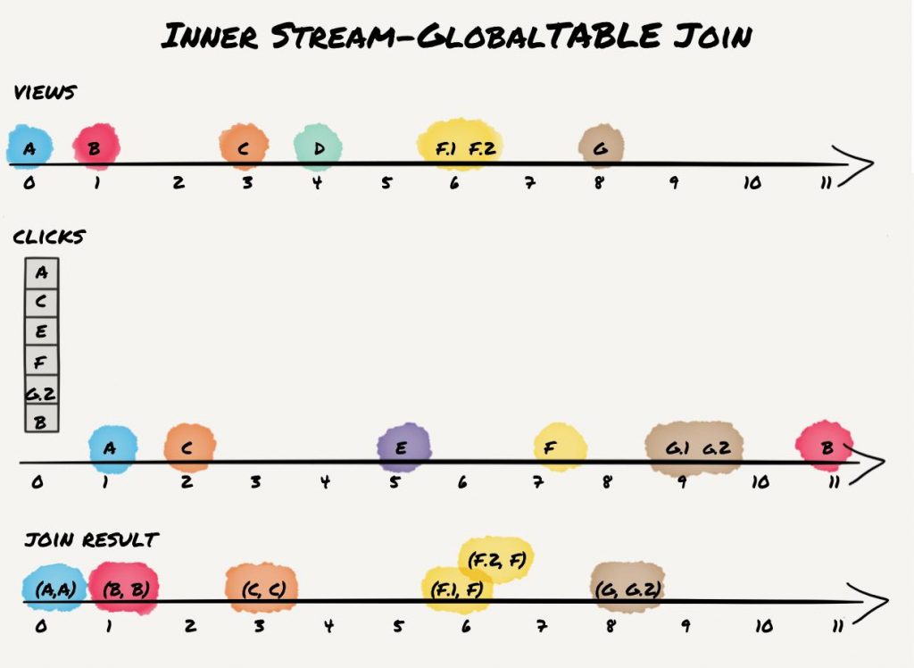
As indicated in the figure, all clicks are first read to populate the global click table. Afterward, view events are processed. Thus, all views except D join. Also note, that view G only joins with G.2 but not with G.1 as G.1 gets overwritten by G.2 while preparing the global table.
Note, that a KStream-GlobalKTable join does not have the same runtime dependency as KStream-KTable joins as the global table is built up completely at startup and before any actual processing begins.
Left KStream-GlobalKTable Join
The last join in the left KStream-GlobalKTable join. The result is as follows:
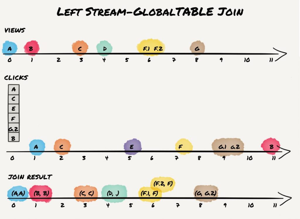
The result is the same as for inner KStream-GlobalKTable join plus the additional left join result for view event D.
Partitioning and Parallelization
If you are familiar with Kafka consumers, you are probably aware of the concept of the consumer groups—Kafka consumption is parallelized by assigning partitions to exactly one consumer in a group of consumers that share the same group id. If you’re using defaults, Kafka itself will handle the distribution and assign the partitions to consumers. This happens in a way that the consumers have little influence over.
With simple consumers, this is quite straightforward. However, what does it mean for a Kafka stream with state and joins? Can partitions still be randomly distributed? No, they cannot. While you can run multiple instances of your streaming application and partitions will be distributed among them, there are requirements that will be checked at startup. Topics that are joined need to be co-partitioned. That means that they need to have the same number of partitions. The streaming application will fail if this is not the case. Producers to the topic also need to use the same partitioner although that is something that cannot be verified by the streaming application as the partitioner is a property of the producer. For example, you will not get any join results if you send view event “A” to partition 0 and the corresponding click event to partition 1 even if both partitions are handled by the same instance of the streaming application.
Using a GlobalKTable frees from the above limitations. Because a GlobalKTable holds a complete copy of all data over all partitions of its input topic, the number of KStream partitions must not match the number of GlobalKTable source topic partitions. Furthermore, the partitioning can be random as co-partitioning is not required. However, the disadvantages of a global table are an increased memory/disk usage as well as a timely decoupling of both streams. While the timely decoupling might seem like an advantage, the drawback is that it makes deterministic reprocessing impossible if the GlobalKTable input topic did change in between. Therefore, it’s recommended to use a GlobalKTable for almost static data only and stick with KTable for dynamic tables.
Summary and Outlook
Apache Kafka’s Streams API provides a very sophisticated API for joins that can handle many use cases in a scalable way. However, some join semantics might be surprising to developers as streaming join semantics differ from SQL semantics. Furthermore, the semantics of changelog streams and tombstone messages (that are used for deletes) are a new concept in stream processing.
Kafka’s journey from Pub/Sub broker to distributed streaming platform is well underway, and our times as engineers are very exciting!
About Apache Kafka’s Streams API
If you have enjoyed this article, you might want to continue with the following resources to learn more about Apache Kafka’s Streams API:
- Get started with the Kafka Streams API to build your own real-time applications and microservices.
- Walk through our Confluent tutorial for the Kafka Streams API with Docker and play with our Confluent demo applications.
References
- The official Kafka Streams API documentation on the Apache Kafka website
- Confluent’s Kafka Streams API documentation
- A GitHub repository with examples for all joins as described in this blog post
- Apache Kafka’s official wiki describing current and past join semantics
- First-hand experience with Kafka as part of the SMACK stack
(1)Note that you might observe a different result stream if you run this example with default configurations due to Kafka Streams internal memory management. If caching is enabled, you most likely don’t get (intermediate) result record G/G.1 and only see “final” result G/G.2 as both computations happen shortly after each other and G/G.2 will overwrite G/G.1 in the cache before the cache gets flushed.
(2) Note, that with old join semantics (before Kafka 0.10.2) a KTable-KTable join did write some more tombstone records to the result. Those tombstone records were not wrong but redundant and thus got removed in 0.10.2. A full comparison of old and new join semantics is provided in the Apache Kafka Wiki.
(3)A GlobalKTable additionally holds a full copy of all partitions in each instance and is not shared/partitioned as KTables. However, this does not have any impact on join semantics and thus we don’t cover this difference in detail.
Get started with Confluent, for free
Watch demo: Kafka streaming in 10 minutes
Ist dieser Blog-Beitrag interessant? Jetzt teilen
Confluent-Blog abonnieren


Introducing Versioned State Store in Kafka Streams
Versioned key-value state stores, introduced to Kafka Streams in 3.5, enhance stateful processing capabilities by allowing users to store multiple record versions per key, rather than only the single latest version per key as is the case for existing key-value stores today...


Delivery Guarantees and the Ethics of Teleportation
This blog post discusses the two generals problems, how it impacts message delivery guarantees, and how those guarantees would affect a futuristic technology such as teleportation.